Ni Yan / AWESCO
doctoral training network
Photo was taken during the AWESCO doctoral training network kick-off
week at the University of Freiburg, 29 February - 4 March 2016. In the
Project Management & Strategic Skills course, the newly recruited
PhD researchers of the network learned, among other, also the basics of
airborne wind energy. Original photo: c160305 Fri_PMSS 052.JPG
Terminology
Velocity is a vector property.
Speed is a scalar property, the magnitude
A kite can be of fixed-wing of soft-wing type.
Terminology
Velocity is a vector property.
Speed is a scalar property, the magnitude
A kite can be of fixed-wing of soft-wing type.
Mathematical notation
Scalars are set in italic: \(a\) ,
\(b\) , \(\rho\) , \(\phi\)
In digital resources, vectors are set in bold roman: \(\vec{v}\) , \(\vec{L}\) , \(\vec{D}\)
In handwritten resources, vectors are overset with an arrow: \(\overset{→}{v}\) , \(\overset{→}{L}\) , \(\overset{→}{D}\)
Units are set in roman: \(\rm m\) ,
\(\rm kg\)
Mathematical functions are set in roman: \(\sin\) , \(\cos\) , \(\max\)
Product of scalars: \(a b\)
Scalar product of vectors: \(\vec{v}\cdot\vec{v} = v^2\)
Cross product of vectors: \(\vec{v} =
\boldsymbol\omega\times\vec{r}\)
Cartesian unit vectors: \(\vex\) ,
\(\vey\) , \(\vez\)
Environmental properties
Ambient wind velocity\[\vvw, \quad {\rm m/s}\]
Air density\[\rho, \quad {\rm kg/m}^3\]
Dynamic wind pressure\[q = \frac{1}{2}\rho\vw^2, \quad {\rm
N/m}^2\]
Wind power density\[\Pw = \frac{1}{2}\rho\vw^3, \quad {\rm
W/m}^2\]
Gravitational acceleration\[\vec{g}, \quad {\rm m/s}^2\]
We use “ambient” to distinguish from the “apparent” wind velocity.
Kite properties
Flat wing surface area (unrolled)
Wing planform area (projected)\[S, \quad {\rm m}^2\]
Wing span\[b, \quad {\rm m}\]
Wing side area (projected)
Wing maximum chord\[\cmax, \quad {\rm m}\]
Airfoil geometry
Kite mass¹\[\mk, \quad {\rm kg}\]
1 Often also just denoted as \(m\) , without subscript.
Example: TU Delft V3 kite
Tethered
static flight
Library of Congress / NPS.gov
Dan Tate, left, and Wilbur Wright, right, flying
https://rarehistoricalphotos.com/first-flight-wright-brothers/
Static massless kite
Kite velocity\[\vvk = 0\]
Apparent wind
velocity\[\vva = \vvw - \vvk =
\vvw\]
Static force
equilibrium\[\vFt + \vFa = 0\]
\[\Ft = \Fa = \sqrt{L^2 + D^2}\]
\[\begin{align}
\tan\beta & = \frac{L}{D} \\
\beta & = \arctan\frac{L}{D}
\end{align}\]
\[\lim_{\frac{L}{D}⤳\infty} \beta =
\frac{\pi}{2}\]
Effect of gravity
Static force equilibrium\[\vFt + \vFa + m\vg = 0\]
\[\Ft = \sqrt{\left(L-mg\right)^2 +
D^2}\]
\[\begin{align}
\tan\beta & = \frac{L-mg}{D} \\
& = \frac{L}{D} \left[1-\frac{mg}{L}\right] \\
& = E\,\left[1-\frac{2gm}{\rho\CL S \vwexp2}\right]
\end{align}\]
\[\begin{align}
\phantom{\tan\beta} & =
E\,\left[1-\frac{\color{red}{\frac{2g}{\rho\CL}\frac{m}{S}}}{\vwexp2}\right]
\end{align}\]
But what is the
physical meaning of \(\color{red}{\frac{2g}{\rho\CL}\frac{m}{S}}\) ?
The formula for the elevation angle is also listed as Eq. (15) in
Snyder, I., Cairncross, R., Bland, G. and Stout, D.: “Using Measured
Aerodynamic Coefficients to Predict Pitch Equilibrium of Kites”. Journal
of Aircraft, pp. 1-7, 2025. https://doi.org/10.2514/1.C038138
Static take-off limit
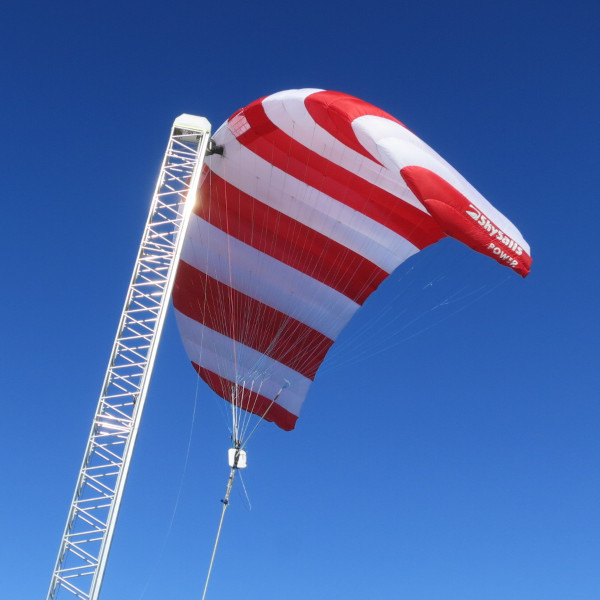
SkySails’ static mast launch
Generated lift just balances the effect of gravity:\[\frac{1}{2}\rho\CL S
\vwexp2=mg\]
Equivalent to \(\beta = 0\)
(horizontal tether).
Solving for \(\vw\) leads to static take-off wind
speed:\[\vwsto =
\sqrt{\frac{2g}{\rho\CL}\frac{m}{S}}\]
Mass-to-area ratio \(m/S\) is an
important scaling parameter affecting take-off limit
Definition identical to the stall speed
\(\vstall\) of an aircraft
(Anderson 2016 ) .
To investigate this, we consider the case where the wind is just
strong enough to lift the kite off the ground. In this condition,
denoted as static take-off limit, the tether is horizontal (\(\beta=0\) ) and the aerodynamic lift force
\(\vec{L}\) exactly balances the
gravitational force \(m\vec{g}\) . In
horizontal direction, the drag force \(\vec{D}\) is balanced by the tether force
\(\vFt\) . The static force equilibrium
in this limiting case is illustrated in the schematic. In practice, this
specific situation occurs during a mast-based launch, as the photo of
the SkySails system shows.
From the vertical force balance, we can derive an expression for the
minimum wind speed required for the kite to statically take off, which
we denote as \(\vwsto\) .
The situation depicted in the schematic is similar to steady levelled
flight of an aircraft, where the thrust force takes the role of the
tether force. This leads to the stall speed \(\vstall\) of an aircraft, which is defined
by the identical expression (Anderson 2016 ) .
Effect of gravity
Static force equilibrium\[\vFt + \vFa + m\vg = 0\]
\[\Ft = \sqrt{\left(L-mg\right)^2 +
D^2}\]
\[\begin{align}
\tan\beta & = \frac{L-mg}{D} \\
& = \frac{L}{D} \left[1-\frac{mg}{L}\right] \\
& = E\,\left[1-\frac{2gm}{\rho\CL S \vwexp2}\right]\\
& =
E\,\left[1-\frac{\color{red}{\frac{2g}{\rho\CL}\frac{m}{S}}}{\vwexp2}\right]
\end{align}\]
\[\begin{align}
\phantom{\tan\beta} & =
E\,\left[1-\left(\frac{\color{red}{\vwsto}}{\vw}\right)^2\right], \quad
\text{with} ~ \vwsto = \sqrt{\frac{2g}{\rho\CL}\frac{m}{S}}
\end{align}\]
The ratio of the wind speed \(\vw\)
and the static take-off wind speed \(\vwsto\) is a non-dimensional parameter.
Its square \(L/(mg)\) quantifies the
relative strength of the aerodynamic lift force compared to the
gravitational force. The threshold value 1 defines the static take-off
limit. The use of force ratios to define non-dimensional parameters is a
useful practice in many engineering disciplines.
The characteristic speed \(\vwsto\)
also affects the dynamic take-off limit, as we will show in short. Luchsinger (2013 ) uses
the ratio of centrifugal force to lift force to derive an expression for
the minimal turning radius that a kite can fly. We will get to this
later.
Static take-off wind speed
Kite
\(S~\text{(m$^\text{2}$)}\) \(m~\text{(kg)}\) \(\CLmax~\text{(-)}\) \(m/S~\text{(kg/m$^\text{2}$)}\) \(\vwsto~\text{(m/s)}\)
Ampyx AP2
3
35
1.5
11.7
11.3
Mozaero AP3
12
475
2.1
39.6
17.5
Makani MX2
54
1850
2
34.3
16.7
MegAWES
150.45
6885
1.9
45.8
19.8
TU Delft V3
19.75
22.8
0.88
1.15
4.6
Kitepower V9
47
73
1.19
1.55
4.6
Source:
Joshi et al. (2024 )
Ideal crosswind
flight
TU Delft V3 kite flying on launch mast in 2012
Massless crosswind kite
Reeling factor ⤳
degree of freedom\[f = \frac{\vkx}{\vw}\]
Tangential velocity
factor\[\lambda =
\frac{\vky}{\vw}\]
Apparent wind
velocity\(\begin{aligned}
\vva & = \vvw - \vvk \\
& = \left( \vw - \vkx \right)\vex + \left( - \vky
\right)\vey
\end{aligned}\)
Geometric similarity
of velocity and force triangles\[\frac{L}{D} = \frac{\vky}{\vw-\vkx} \qquad
⤳ \qquad \frac{L}{D}\left( \vw - \vkx \right) = \vky \\
\lambda = \frac{L}{D} \left( 1-f \right) = E \left( 1-f \right)
\quad \quad \text{dependent variable, i.e. not a degree of
freedom!}\]
Massless crosswind kite
Apparent wind velocity\(\begin{aligned}
\vaexp{2} & = \left( \vw-\vkx \right)^2 + \vky^2 \qquad ⤳ \qquad
\left(\frac{\va}{\vw}\right)^2 = \left( 1-f \right)^2 + \lambda^2\\
\frac{\va}{\vw} & = \left( 1-f \right) \sqrt{1+E^2}
\end{aligned}\)
Aerodynamic
force\[\Fa = \frac{1}{2}\rho S \CR \vaexp{2} =
\frac{1}{2}\rho S \CL \sqrt{1+\frac{1}{E^2}}
\left(\frac{\va}{\vw}\right)^2 \vwexp{2}\]
Non-dimensional tether
force\[\frac{\Ft}{qS} = \CL \sqrt{1+\frac{1}{E^2}}
\left( 1-f \right)^2 \left( 1+E^2 \right), \quad \text{with} \qquad
q=\frac{1}{2}\rho\vwexp{2}\]
Power harvesting
factor\[\zeta = \frac{P}{\Pw S} = C_L
\sqrt{1+\frac{1}{E^2}} f \left( 1-f \right)^2 \left( 1+E^2 \right),
\quad \text{with} \qquad \Pw =
\frac{1}{2}\rho\vwexp{3}\]
Optimal reel-out speed
Maximum power harvesting factor at maximum value of\(f \left( 1-f \right)^2\)
This leads to a
condition for the first derivative\[0 = \frac{\rm{d}}{\rm{df}} \left[ f \left(
1-f \right)^2 \right]\]
from which the optimal
reeling factor can be determined\[\fopt=\frac{1}{3}\]
Optimal harvesting
factor using \(\fopt\) \[\zetaopt = \frac{4}{27} C_L
\sqrt{1+\frac{1}{E^2}}\left( 1+E^2 \right)\]
Reality check
The analytic formula for \(\zetaopt\) is based on a number of
idealizations :
ideal crosswind operation at \(\beta=\phi=0\) ,
neglected reel-in phase,
vanishing mass of the airborne system components,
dragless tether.
In reality, the achievable power harvesting
factor is substantially lower than predicted by \(\zetaopt\) .
Compare achievable power harvesting factor of the Kitepower Falcon :
rated power of 100 kW at the rated wind speed of 10 m/s,
optimal power harvesting factor \(\zetaopt=\) 11.36,
achievable power harvesting factor \(\zeta=\) 3.47.
This is about 30% of the theoretical optimum
value.
Maximum reel-out factor?
At \(f=1\) the apparent wind speed
vanishes
But what happens for \(f>1~(\vt>\vw)\) ?⤳ gliding in downwind
direction, ⤳
vanishing tether tension.
Practical application is step towing ,
bydownwind gliding with \(f>1\) , andupwind
retraction of the kite with \(f<0\) .
Technique well known from winch
Note: for \(\beta>0\) and/or \(\phi \ne 0\) , \(\va\) vanishes for \(f<1\) .
Crosswind kite with mass
Static force equilibrium\[\vFt + \vL + \vD + m\vg = 0\]
Horizontal lift force
component\[|\vec{L} + m\vec{g}| = \sqrt{L^2 -
\left(mg\right)^2}\]
Geometric
similarity\[\frac{\vky}{\vw-\vkx} = \frac{\sqrt{L^2 -
\left(mg\right)^2}}{D}\]
Tangential velocity
factor\[\lambda = (1-f)E\sqrt{1 - \left(
\frac{mg}{L} \right)^2}\]
2025-04-10-resit
Crosswind kite with mass
Apparent wind speed\[\begin{align}
\left( \frac{\va}{\vw} \right)^2 & = (1-f)^2 + \lambda^2 \\
& = \left( 1 - f \right)^2 \left\{
1 + E^2\left[ 1-\left(\frac{mg}{L}\right)^2 \right] \right\} \\
& = \left( 1 - f \right)^2 \left\{
1 + E^2\left[
1-\left(\frac{\frac{2g}{\rho\CL}\frac{m}{S}}{\vaexp{2}}\right)^2 \right]
\right\}
\end{align}\]
Substitute\[\color{red}{x} = \left( \frac{\va}{\vw}
\right)^2\quad ⤳\]
\[\color{red}{x} = \left( 1 - f \right)^2 \left\{ 1
+ E^2\left[ 1-\left(\frac{\vwsto}{\vw}\right)^4
\frac{1}{\color{red}{x^2}}\right]\right\}\]
2025-04-10-resit
Crosswind kite with mass
\[\color{red}{x} = \left( 1 - f \right)^2
\left\{ 1 + E^2 - E^2\left(\frac{\vwsto}{\vw}\right)^4
\frac{1}{\color{red}{x^2}}\right\}\]
Cubic equation, with missing linear term\[\color{red}{x^3} - \left( 1 - f \right)^2
\left( 1 + E^2 \right) \color{red}{x^2} + \left( 1 - f \right)^2 E^2
\left(\frac{\vwsto}{\vw}\right)^4 = 0\]
Cubic equation in standard form\[a x^3 + b x^2 + c x + d = 0, \quad
\text{with}\]
\[\begin{align}
a & = 1, \\
b & = - \left( 1 - f \right)^2 \left( 1 + E^2 \right), \\
c & = 0, \\[-15px]
d & = \left( 1 - f \right)^2 E^2 \left(\frac{\vwsto}{\vw}\right)^4.
\\
\end{align}\]
2025-04-10-resit
One can recognize the effect of mass in the constant term of the cubic
equation. With \(m \to 0\) , also \(\vwsto \to 0\) and the constant term
vanishes, recovering Loyd’s ideal crosswind case, \(x=\left( 1 - f \right)^2 \left( 1 + E^2
\right)\) .Niccolò
Tartaglia in 1530 (Kichenassamy 2015 ) . In 1539, he revealed
the solution to his contemporary Gerolomo
Cardano , who included it in his 1545 book Ars
Magna , which also described the solution of the general cubic
equation. The historical developments are described in more detail in this
article .
Number and nature of roots
A cubic equation has three roots. The nature of the three roots
depends on the value of the discriminant\[
\begin{align*}
\Delta & = \ccancel{18 abcd} - 4b^3d + \ccancel{b^2c^2} -
\ccancel{4ac^3} - 27 a^2d^2 \fragment{0}{, \quad \text{because} \quad
\color{red}{c=0}} \\
& \fragment{1}{{} = 4(1-f)^8(1+E^2)^3 E^2 \left(
\frac{\vwsto}{\vw} \right)^4 - 27(1-f)^4 E^4 \left( \frac{\vwsto}{\vw}
\right)^8,} \\
& \fragment{2}{{} = (1-f)^4 E^2 \left( \frac{\vwsto}{\vw}
\right)^4 \left[ 4 (1-f)^4 (1+E^2)^3 - 27 E^2 \left( \frac{\vwsto}{\vw}
\right)^4 \right]}
\end{align*}
\]
For \(\Delta < 0\) , the equation
has one real root and two non-real complex conjugate roots.
For \(\Delta = 0\) , the equation has
one real root and two real repeated roots.
For
\(\Delta > 0\) , the equation has
three distinct real roots.
Cubic polynomial
Polynomial function and derivatives\[\begin{alignat*}{2}
&p(x) &&= x^3 - \left( 1 - f \right)^2 \left( 1 + E^2
\right) x^2 + \left( 1 - f \right)^2 E^2
\left(\frac{\vwsto}{\vw}\right)^4, \\[-6mm]
&p'(x) &&= 3x^2 - 2\left( 1 - f \right)^2 \left( 1 +
E^2 \right) x, \\
&p''(x) &&= 6x - 2\left( 1 - f \right)^2 \left( 1 +
E^2 \right).
\end{alignat*}\]
⤳ Wind speed \(\vw\) affects
vertical offset of polynomial
End behavior\[\begin{alignat*}{3}
&x\to & -\infty &⤳ p(x)\to & ~ -\infty, \\
&x\to & \infty &⤳ p(x)\to & ~ \infty.
\end{alignat*}\]
Critical points: local
extrema \((p'=0)\) \[\begin{alignat*}{4}
&x &&
=0 &&⤳
\text{local maximum} && (p'' < 0). \\
&\xc && =\frac{2}{3} \left( 1 - f \right)^2 \left( 1 + E^2
\right) &&⤳ \text{local minimum} \quad && (p''
> 0).
\end{alignat*}\]
Polynomials for the TU Delft V3 kite at \(f=0\) .
From the first and second derivatives of this specific cubic polynomial
it is clear that the wind speed only affects the vertical offset of the
curve, while the ploynomial’s shape is not affected. Increasing wind
speeds \(\vw\) shift the polynomial
curve to lower values of \(x\) and thus
lower values of \(p(x)\) .\(x\) ,
the polynomial \(p(x)\) is negative,
while for sufficiently large \(x\) , the
polynomial is positive.\(x=0\) , the polynomial exhibits a
local maximum (\(p''<0\) )
while the function value \(p=(1-f)^2 E^2
\left( \vwsto/\vw\right)^4\) is positive. This means, the
polynomial curve needs to cross the negative \(x\) -axis, which means that one real root is
always negative. The other two real roots (intersections of the
polynomial with the \(x\) -axis) either
do not exist, as illustrated here for the case \(\vw=1/4\vwsto\) , or do exist, as
illustrated here for the two higher \(\vw\) -cases.\(\xc\) , the polynomial \(p(x)\) exhibits a local minimum (\(p''>0\) ).
Physical solution space
\(x \ge \xmin = (1-f)^2.\)
This lower limit follows from the definition of the
non-dimensional apparent wind speed as\[x = (1-f)^2+\lambda^2,\]
and the fact that the crosswind contribution is always positive,
i.e. \(\lambda^2 \ge 0\) .
\(x \le \xmax = \left( 1 - f \right)^2 \left(
1 + E^2 \right).\)
This upper limit is the apparent wind speed for Loyd’s ideal crosswind case, where \(m=0\) .
Interesting is also the observation
\[\xc = \frac{2}{3} \xmax.\]
Polynomials for the TU Delft V3 kite at \(f=0\) .
The physical solution space is smaller than the mathematical solution
space. In other words, not all mathematical solutions are physically
meaningful. The physical limits of the mathematical solution space can
be derived from additional conditions.\(\lambda^2 \ge 0\) . The lowest possible,
physically meaningful value of \(x\) is
thus given by \(\lambda=0\) . This
corresponds to a lower physical limit for the non-dimensional apparent
wind speed of \(\left( \va/\vw
\right)_\mr{min}=1-f\) .\(p(x)\) occors exactly at two thirds of the
maximum value.
Minimum flyable wind speed
At \(\vw=\frac{1}{4}\vwsto\) , the cubic equation
has no real roots in the physical solution space.
At \(\vw=\frac{1}{3}\vwsto\) , the cubic equation
has two real roots in the physical solution space.
At what value of \(\vw\) does the cubic equation have a
repeated real root , transitioning from no real root to
two real roots?
This transition is described mathematically by the
discrimonant \(\Delta\) changing the
sign from negative to positive.
Polynomials for the TU Delft V3 kite at \(f=0\) .
Discriminant
The discriminant is positive when\[
\begin{align*}
4 (1-f)^4 (1+E^2)^3 & > 27 E^2 \left(
\frac{\vwsto}{\vw} \right)^4, & & \\
\fragment{0}{{}\left( \frac{\vw}{\vwsto} \right)^4} &
\fragment{0}{{} > \frac{27 E^2}{4 (1-f)^4 (1+E^2)^3},} & & \\
\fragment{1}{{}\vw} &
\fragment{1}{{} > \sqrt[\Large 4]{\frac{27 E^2}{4(1+E^2)^3}}
\frac{\vwsto}{1-f},} & \\
\fragment{2}{{}\vw} &
\fragment{2}{{} > \frac{\vwc}{1-f}, \quad \text{with} \quad}
&
\fragment{2}{{} \vwc } & \fragment{2}{{} = \sqrt[\Large 4]{\frac{27
E^2}{4(1+E^2)^3}}\, \vwsto, \quad \text{and}} \\
& &
\fragment{2}{{} \vwsto} & \fragment{2}{{} =
\sqrt{\frac{2g}{\rho\CL}\frac{m}{S}}.}
\end{align*}
\]
But what is the
physical meaning of \(\vwc\) ?
Cubic polynomial
Polynomial for \(f=0\) and physical
parameters of the TU Delft V3 kite
Investigate the cubic polynomial for\(\vw=\) \(0.9\vwc\) , \(\vwc\) and \(1.1\vwc\) .
By definition \(x = \left( \frac{\va}{\vw} \right)^2 \ge
0\) ,\(x<0\) unphysical.
For \(\vw<\vwc\) \((\Delta < 0)\) ,
For \(\vw=\vwc\) \((\Delta = 0)\) ,
For \(\vw>\vwc\) \((\Delta > 0)\) .
Only interested
in the lower value.
Because of the missing linear term (\(c=0\) ), the first derivative of the cubic
polynomial is zero at \(x=0\) , which
means that the local maximum of the polynomial is always at \(x=0\) .\(\Delta=0\) .
Full wind speed range
Tangential velocity factor \(\lambda_\mathrm{max} = \lambda(m=0)= E\) .
These diagrams illustrate the solutions of the force equilbrium: the top
diagrams show the required apparent wind speed, while the bottom digrams
show the required flight speed of the kite. The static take-off limit at
\(\vwsto\) is characterized by \(\va/\vw=1\) , where \(\vk=0\) and \(\va=\vw\) .
Interpretation
Considering a kite with a static take-off wind
speed \[\vwsto =
\sqrt{\frac{2g}{\rho\CL}\frac{m}{S}},\]
the theoretical cut-in wind speed for crosswind
operation at \(\beta=\phi=0\) is given
by\[\vwc = \sqrt[\Large 4]{\frac{27
E^2}{4(1+E^2)^3}}\, \vwsto.\]
This definition of a lower wind speed limit implies a constant
tether length (\(f=0\) ).
For \(\vw < \vwc\) , the kite can
not generate a sufficient lift force for sustained flight.
For \(\vwc < \vw < \vwsto\) ,
the generated lift force can counteract gravity. In this wind speed
regime, the tangential velocity factor \(\lambda\) is a function of the wind speed
\(\vw\) .
For \(\vw > \vwsto\) , the
generated lift force is too high, driving the kite to a force
equilibrium at higher elevation angles \(\beta\) , or requiring reeling out (\(f>0\) ).
Interpretation
By reeling in (\(f<0\) ), the
flyable wind speed range can be temporarily decreased below the value of
\(\vwc\) , however, this condition can
not be maintained for longer time.
This low wind speed regime is particularly important for dynamic
launching of kites.
While the static take-off wind speed \(\vwsto\) is affected by the lift
coefficient \(\CL\) , the theoretical
cut-in wind speed \(\vwc\) adds the
dependence on the lift to drag ratio \(E\) .
Static take-off wind speed is affected by mass scaling,
predominantly via the ratio \(m/S\) .
Theoretical cut-in wind speed is substantially lower, especially for
kites with high aerodynamic performance \(E=L/D\) .
The analysis is highly idealized and the real cut-in wind speed of
the kite will be higher.
Approximation
For \(E \gg 1\) the expression for
\(\vwc\) can be approximated\[\begin{align}
\vwc & = \sqrt[\Large 4]{\frac{27 E^2}{4(1+E^2)^3}}\, \vwsto, \\
& = \sqrt[\Large 4]{\frac{27}{4}}\, \frac{1}{E}\, \vwsto, \\
& = \frac{1.612}{E}\, \vwsto.
\end{align}\]
Radial flight
Because the tether force is much lower in this flight mode, the
gravitational loading of the tether leads to a much more pronounced
sagging than for crosswind flight. Also, the kite (considered as
assembly of wing, bridle line system and kite control unit)
As expected, the tether is sagging much
Massless radial kite
Reeling factor ⤳
degree of freedom\[f = \frac{\vk}{\vw}\]
Apparent wind
velocity\[\vva = \vvw - \vvk\]
Decomposition of kite
velocity\[\vvk = \vec{b} + \vec{c}\]
\[\vva = \vvw - \vec{b} - \vec{c}\] \[\vvw = \vva + \vec{c} + \vec{b}\] \[\vw^2 = \left( \va - c \right)^2 + b^2\quad
\text{(positive vector magnitudes!)}\] \[\frac{\va}{\vw} =
\sqrt{1-\left(\frac{b}{\vw}\right)^2} +
\frac{c}{\vw}\]
Displayed is the case for reel in with \(f<0\)
Massless radial kite
Geometric similarity\[\frac{b}{\vk} = \frac{L}{\Fa} =
\frac{1}{\sqrt{1+\frac{1}{E^2}}}\] \[\frac{c}{\vk} = \frac{D}{\Fa} =
\frac{1}{\sqrt{1+E^2}}\]
Normalized to the wind speed\[\frac{b}{\vw} =
-\frac{f}{\sqrt{1+\frac{1}{E^2}}}\] \[\frac{c}{\vw} =
-\frac{f}{\sqrt{1+E^2}}\]
Minus signs aacount for negative value of
\(f\)
Displayed is the case for reel in with \(f<0\)
Massless radial kite
Apparent wind speed\[\begin{align}
\frac{\va}{\vw} & = \sqrt{1 - \frac{f^2}{1 + \frac{1}{E^2}}} -
\frac{f}{\sqrt{1 + E^2}}, \\
& = \frac{\sqrt{1 + E^2\left( 1 - f^2 \right)} -
f}{\sqrt{1 + E^2}}
\end{align}\]
Non-dimensional tether force\[\frac{\Ft}{qS} = \CL
\frac{\left[\sqrt{1+E^2(1-f^2)}-f\right]^2}{E\sqrt{1+E^2}}\]
Power harvesting factor\[\zeta = \CL
\frac{f\left[\sqrt{1+E^2(1-f^2)}-f\right]^2}{E\sqrt{1+E^2}}\]
Displayed is the case for reel in with \(f<0\)
Massless radial kite
Elevation angle ⤳ not a degree of freedom\[\cos\beta =
\frac{\sqrt{1+E^2(1-f^2)}+fE^2}{1+E^2}\]
Homework #1: Derive this expression.
Hint:
Formulate two different expressions for the apparent wind speed, one
of them containing \(\cos\beta\) .
Eliminate the apparent wind speed by equating those equations.
Solve for \(\cos\beta\) .
2022-04-06-resit
2(d)
Massless radial kite
Minimum reeling factor\[f_{\rm
min}=-\sqrt{1+\frac{1}{E^2}}\]
Homework #2:
Hint:
Use the fact that the radicant in the expression for \(\cos\beta\) has to be greater or equal to
zero.
2022-04-06-resit
2(f)
How to use these analytic models?
The wind speed \(\vw\) describes the available energy
resource. The lift-to-drag ratio \(E\) characterizes the specific kite
design.
For the ideal crosswind kite
prescribe
the tether reeling speed \(\vt\) to calculate the achievable kite
crosswind speed \(\vkx\) ,
or the kite crosswind speed \(\vkx\) to calculate the required tether
reeling speed \(\vt\) .
For the non-maneuvering kite
prescribe
the tether reeling speed \(\vt\) to calculate the achievable elevation
angle \(\beta\) , or the elevation angle \(\beta\) to calculate the required tether
reeling speed \(\vt\) .


